Creating a PWHL model: what are expected goals?
phwl
modeling
the best way to learn about expected goals is to make 8 models
This is a series of posts in which I create an open-source PWHL model. We’ll calculate expected goals in various ways, create forecasts, and explore other things we could do with the model, like player ratings. If this sounds fun, you can follow along on Github here. When it’s ready and the PWHL season has begun, I’ll have a way to view and interact with the model on my website.
Earlier this year, I decided it would be fun to make a PWHL model. Almost immediately, I also decided that the core of the model would be expected goals. xG is the foundation of the much-memed Deserve to Win O’Meter, as well as other modeling efforts like the now-defunct FiveThirtyEight soccer model. I highly recommend reading how the FiveThirtyEight soccer model works, for game-by-game predictions anyway, because that is the kind of model I will be implementing here.
There are several reasons to use xG. Most important for my purposes, xG tends to be interpretable, is superficially easy to define and explain, and serves as a robust and convenient metric for building win probability models. But you’ll notice I said that xG is only superficially easy to define and explain. In most websites and media spaces, you’ll see a definition of xG that goes something like this:1
Expected Goals is a measure of how many goals a team is expected to score, on average, over a large sample of games. Each shot has an xG value between 0 and 1. For example, a shot with 0.3 xG would be expected to result in a goal 30% of the time.
This is, on its surface, a fine definition. When readers see a stat line like “Boston had 1.5 expected goals on Thursday night versus Montreal’s 4.5”, they know what it means. But that makes it more of an explanation of how to interpret xG, is not a true definition. What we lack from this explanation is a sense for what expected means. Put simply, expected goals are expected according to what, and whom, exactly?2
The first step to making an xG model is define xG specifically enough to allow us to calculate xG. Then we can apply the results in whatever ways we would like to for modeling or ad-hoc data analysis. Definitions are easier to understand in practical terms first, though, so we’ll start there and come back to our definition.
Part 1: The data and the definition
To support the PWHL model, I collected publicly available play-by-play data3 from every PWHL game this past season, including preseason and playoffs. The play-by-play data tracks every shot on goal and seems to include some blocked shots, but it doesn’t have all shot attempts. Because the data isn’t as complete or thorough as NHL data, we can’t make a model as fancy as what exists at The Athletic or Moneypuck.
Our sample consists of roughly 6700 shots (about 5500 on net and 1200 blocked). The play-by-play data contains details for each shot, including the shooter, goaltender, shot location, shot type, shot quality (sort of, we’ll get to this later) and, of course, whether it was a goal.
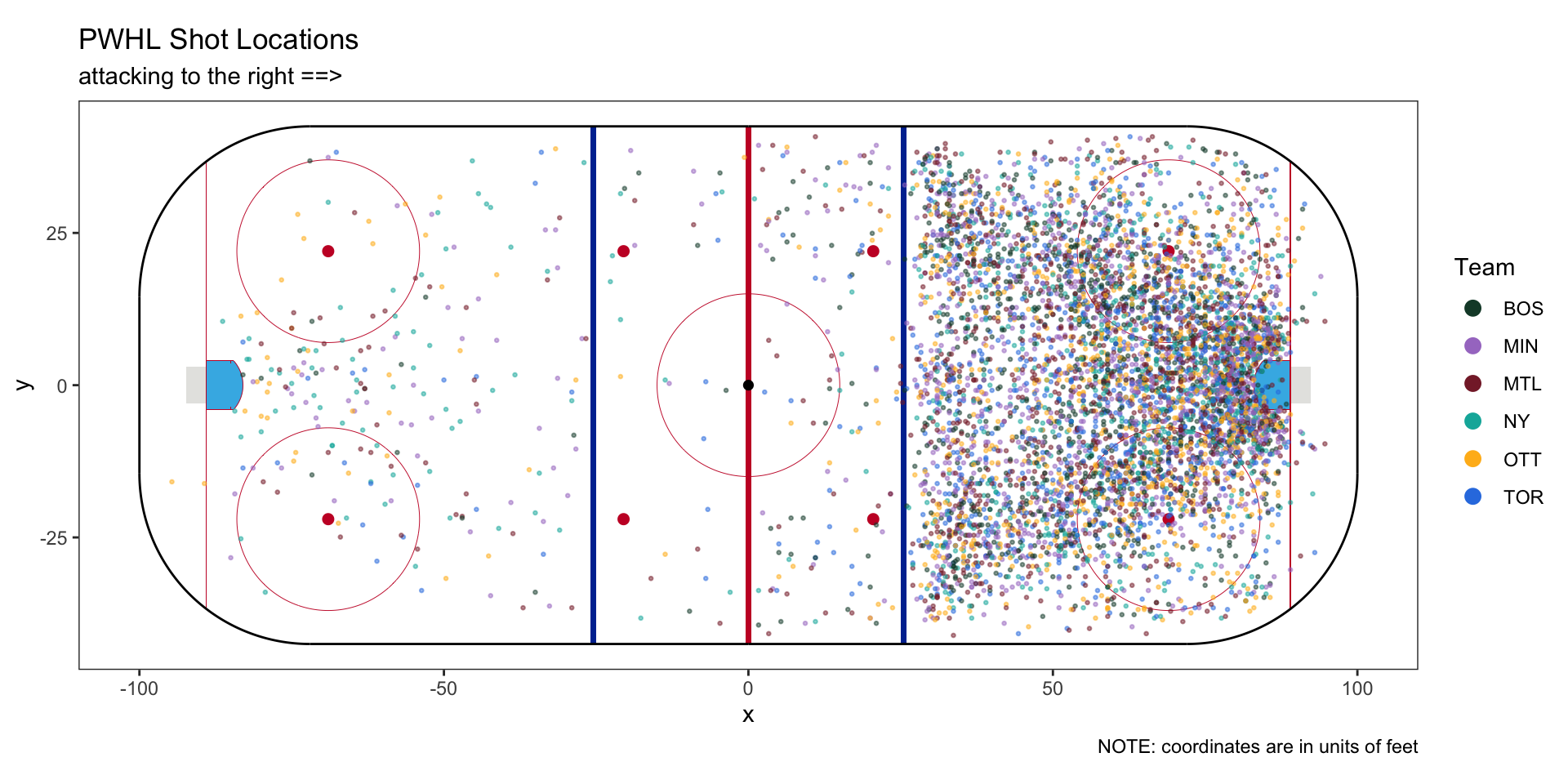
The first thing to do with new data is to plot it. The PHWL data uses coordinate system that ranges from 0 to 300 on the long side of the ice and 0 to 150 on the short side. This conversion is close to 4 inches per unit, but not exactly. I converted everything to units of feet with the origin of our coordinate system at center ice. Then, I flipped the coordinates of half of the data to make it so all shots are attacking the same net.4
This is all we need to make several xG models, except we still lack a workable definition. The definition I shared earlier is incomplete, but it is a good starting point. Specifically, consider the last sentence:
For example, a shot with 0.3 xG would be expected to result in a goal 30% of the time.
How does an expected goals model come to believe a shot has 0.3 xG?
I summarize the answer in 2 steps: Categorize then Count. First, xG models categorize shots from historical data into groups based characteristics have in common.5 Then they count the number of shots and goals in each group and divide the two. The result of that division is the expected goal value.
When an xG model says a shot has 0.3 xG, it’s saying two things. First, it grouped the shot in question with other historical shots based on some of its characteristics. Second, 30% of those historical shots turned into goals. Therefore, the shot in question has 0.3 xG.
This is a functional definition, so the easiest way to truly understand it is to put it into practice. It’s time to create some models.
Part 2: Making models
We now know that the math needed to make an xG model is easy once we choose how to categorize our shot data. For our first model, it makes sense to start with the simplest possible categorization. See if you can figure it out - what’s the smallest possible number of categories needed to make a functional xG model?
Did you guess 0?
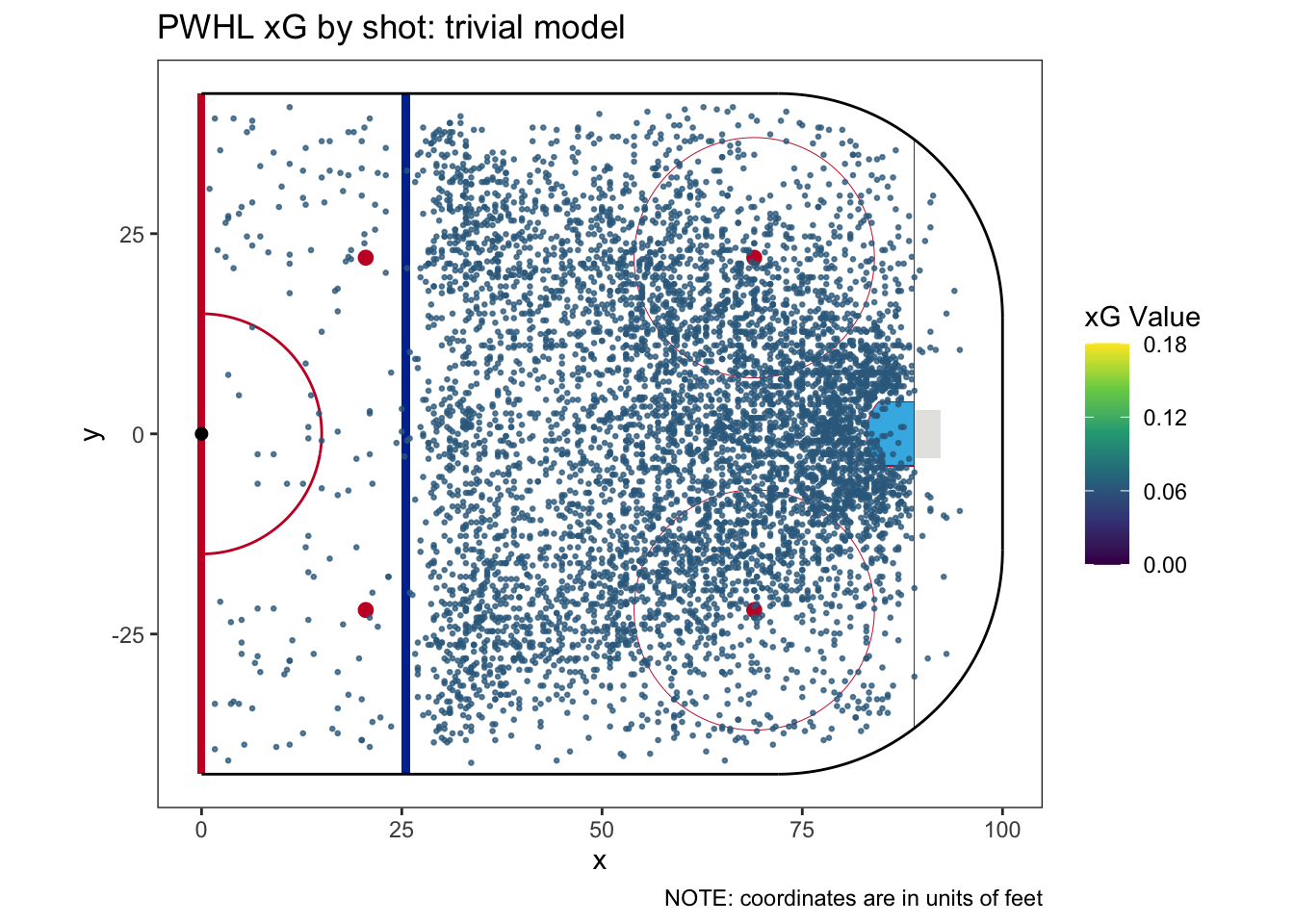
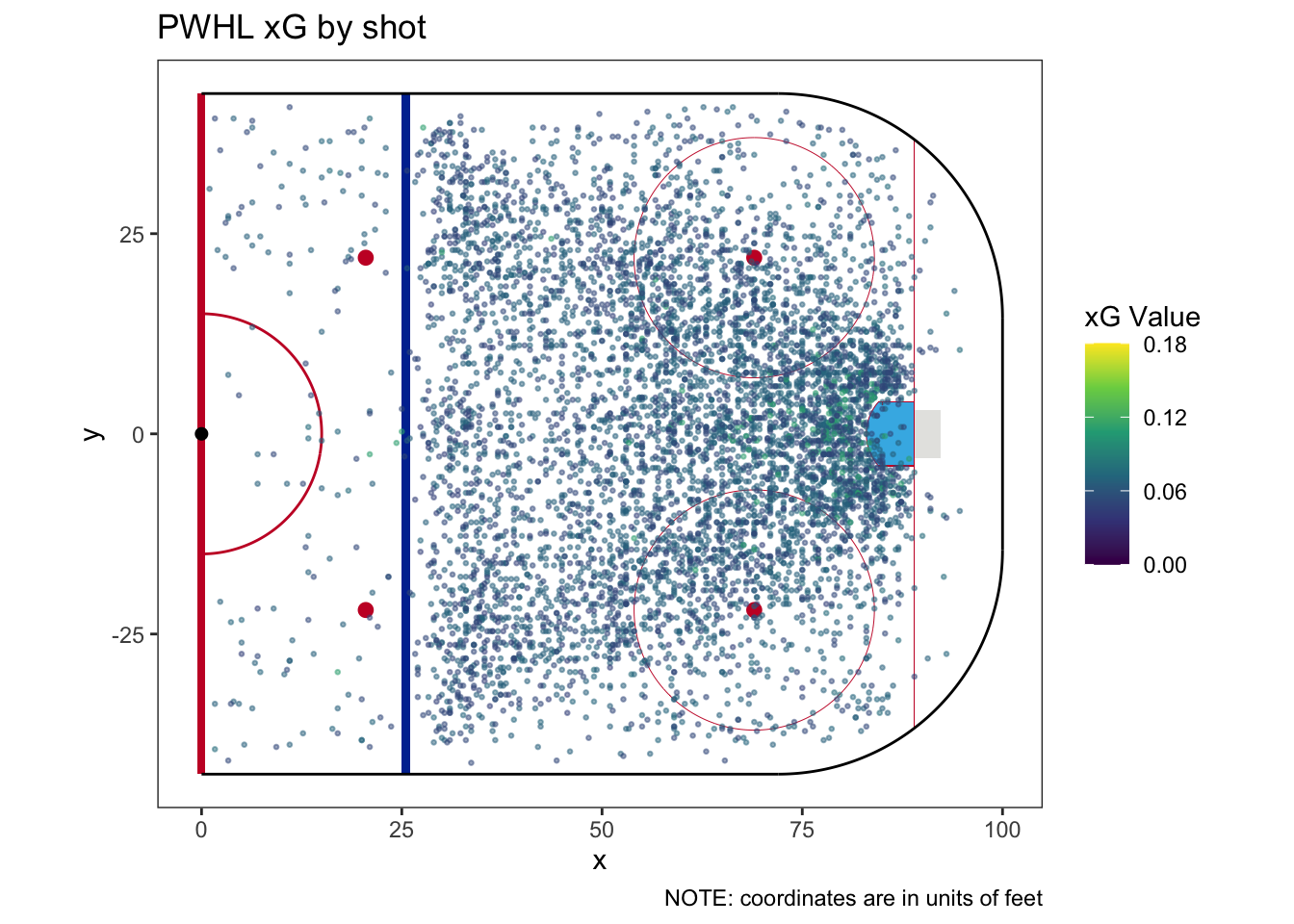
An xG model that doesn’t categorize shots makes a simple claim: a shot is a shot is a shot is a shot. Excluding empty net data,6 our data sample consists of 6,687 shots and 419 goals. This calculates to a shooting percentage of 6.266%, so we assign each shot an xG value of 0.06266.7 Needless to say, this is not a complicated model - in fact, we’ll name this model the trivial model. To see how simple it is, we can plot the data colored by xG value and we’ll only see one color:
To move beyond the trivial model, we’ll start using some shot characteristics. I think there are 4 data points for each shot on which we could build a model - shot type, shooter position (forward or defense), shot quality (such as it exists in the data), and, of course, shot location.
We start with the reported shot type. Intuitively, we may expect that certain shot types are more likely to result in goals than others, so it’s reasonable to calculate xG on this basis. The coded shot types include slap shots, wrist shots, snap shots, backhand shots, and tipped shots. Many shots aren’t coded at all, using a fallback type called default. The following figure shows the xG values for each shot type on the top with the sample size for each shot on the bottom. For reference, the horizontal dashed line represents the trivial model’s xG value.
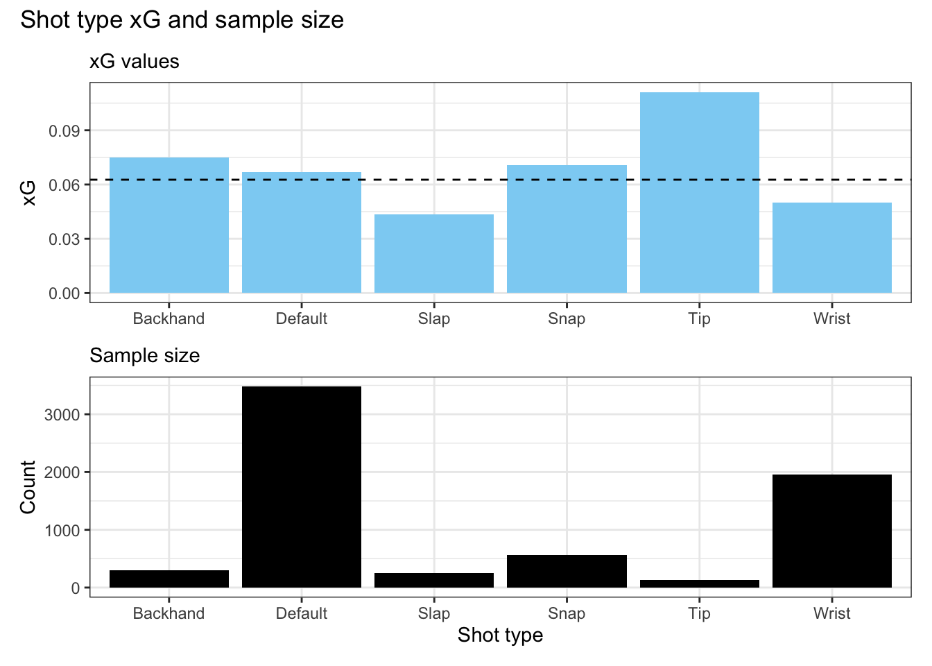
Despite their relative rarity, what jumps out right away is that tipped shots are the most valuable shot type. This aligns with our experience watching the games. An xG model which accounts for shot type using this data would assign an xG value to tipped shots that is about double what they would get in the trivial model. I have a second observation that may be a topic for a future post - the majority of shots in the data are coded with the fallback “default” shot type.
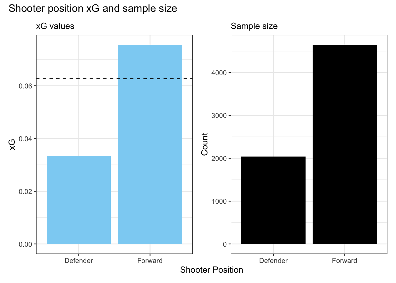
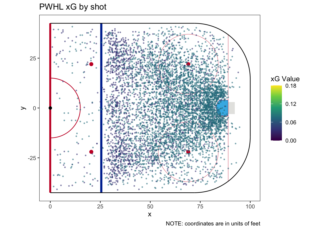
In addition to shot type, it may be useful to know who is taking the shot. Expected goal models generally shouldn’t try to categorize shots by individual players,8 but we can account for position. We may expect forwards, who are mostly responsible for offense, to have a higher collective shooting percentage than defenders. We can see this in the following figure.
Our next characteristic is shot quality. I couldn’t find any documentation on what constitutes a quality shot in the data, but it’s there and may be helpful.
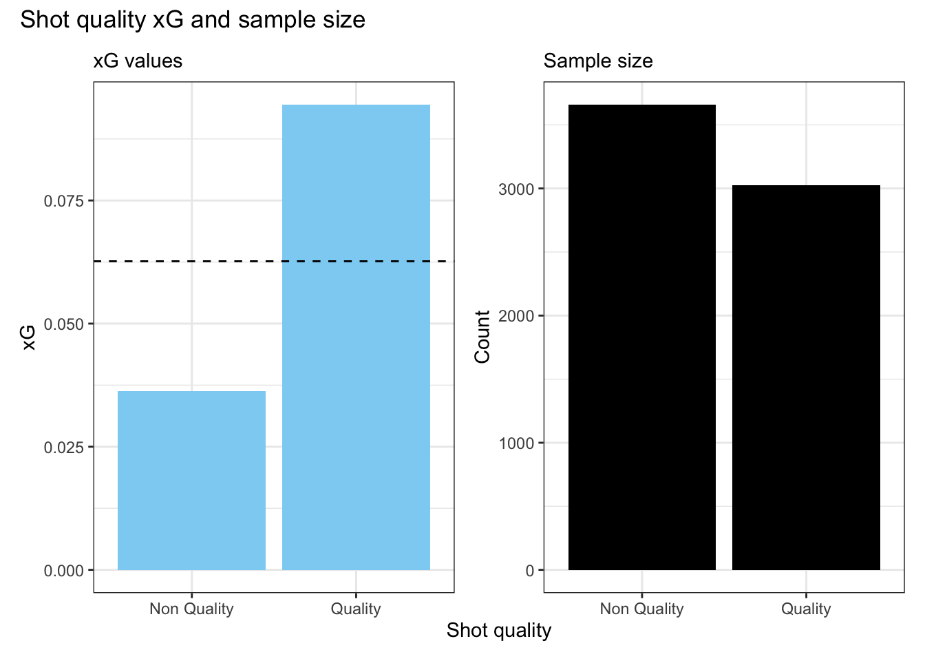
Clearly, the quality indicator is meaningful. Quality shots are about almost 3 times more likely to be goals than non-quality shots, and this is based on a large sample of shots for both categories. Any time there’s an effect size this large, we can be confident there’s something real in the data. Lacking documentation, can we figure out what makes a shot a quality shot?
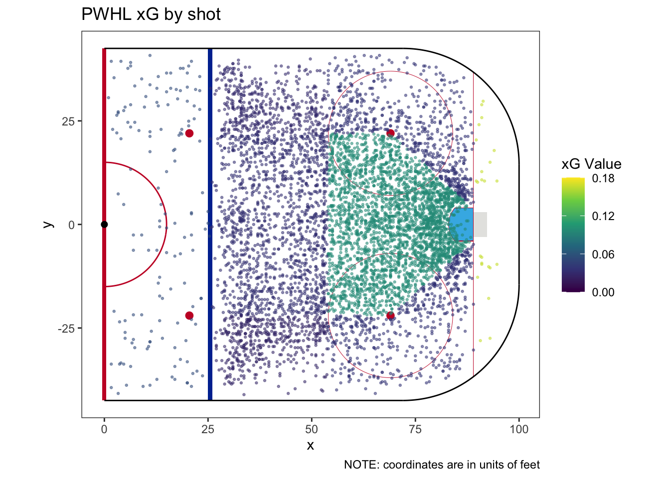
On a hunch, I think we should start by plotting each shot in this model, colored by whether it is quality or not.
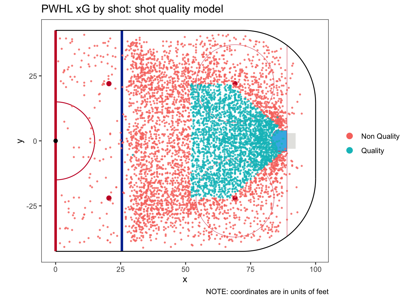
It’s very easy to see what’s going on here. The PWHL shot data is coded for quality based on whether the shot comes from the “home plate” area. The “home plate” area is well-known in hockey analytics. It extends from the edges of the crease to the faceoff dots, and then up to the top of the faceoff circles. This leads us to our next shot characteristic: shot location. We now know that, by definition, it will also cover the shot quality characteristic.
I saved shot location for last because it is the most complicated one to categorize. Unlike the earlier shot characteristics, shot location is based on an x and y coordinate which are continuous variables, not categorical. If we see a shot from, say, x=25.5 and y=18.6, we can’t simply find all the past shots from that spot because chances are very few shots have previously been taken from that exact spot on the ice, if any.
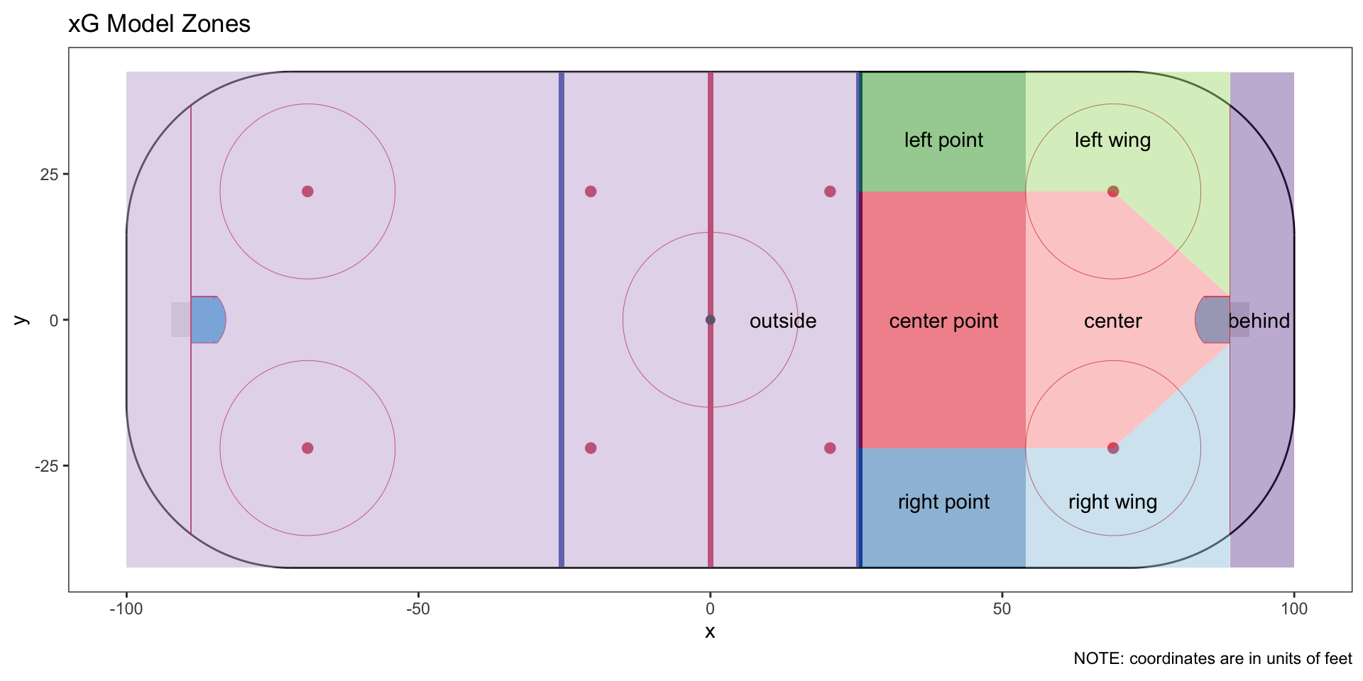
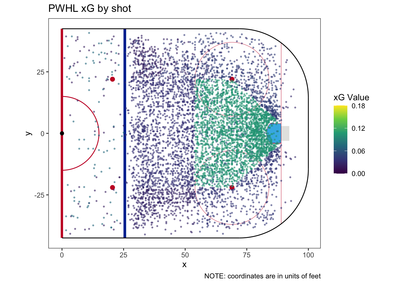
To make an xG model from shot location, we first need to convert it from being continuous to being categorical, a process called discretization. There is no standard or best way to do discretize data. Proper discretization balances the need to have a granular model with the need for a large enough sample in each bin to be statistically meaningful. I landed on having 8 discrete bins, but most xG models have more because they have more data.9
The 8 areas are based on the geometry of the ice. Most notably, I retain the “home plate” shape of the center of the offensive zone, which matches the shot quality flag already coded in the data. I added 5 surrounding segments based on the geometry of the ice, and then two more - one for all shots from behind the net, and the last for all shots outside the offensive zone.
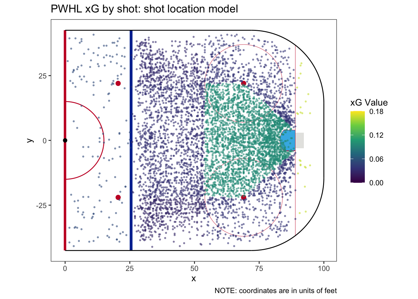
We can see each of the areas clearly if we plot every shot colored by its resulting xG value.
In total, we have 3 possible shot characteristics upon which we can build xG models or, in other words, categorize and then count the shots. We have 6 shot types, 2 shooter positions, and 8 shot location areas. In theory, this means we can have an xG model with anywhere between 0 (the trivial model) and 96 categories. We will be making every model in a bit, but we still have some issues to sort out.
It may be tempting to think that the xG model with the greatest number of categories (more detail) would be the best. But this is not necessarily the case. It’s time to go beyond our definition of an xG model and think about what makes a good xG model. We need to consider two model features I call bounding and resolution. A model with good bounding ensures every possible shot gets an xG value that is reasonable and makes sense (or, in other words, within the bounds of xG). A model with good resolution has a precise understanding of the xG of every shot.10
We’ll start with bounding. From our earlier explanation of xG, we know that the xG value of any shot is between 0 and 1. To be more precise, we should specify that the xG value of any shot should be between 0 and 1 but never exactly 0 or exactly 1. Every shot, theoretically, has some chance of being scored and some chance of being saved, no matter how unlikely. If an xG model categorizes shots and there were no goals for at least one category, it would erroneously assign 0 xG to a future shot. This is poor bounding.
Resolution is a bit tougher to understand theoretically, so we’ll start with a functional example. Imagine an xG model has a category for which its historical sample contains 10 shots. This means that it can only assign 10 possible xG values for this category - 0 if the sample has no goals, 0.1 if the sample has 1 goal, 0.2 for 2 goals, and so on. Resolution is the change in xG observed within a category if its number of goals increases by 1. Our 10-shot category has a resolution of 10%. If the category had 100 shots, its resolution would be 1%. A smaller resolution is better. An xG model has good resolution when all of its shot categories also have good resolution.
As with discretization, there is no single standard for what constitutes good resolution. It’s a balancing act. Setting the bar too high for resolution results in a model with fewer categories and less detail. Setting the bar too low results in a model reporting xG values which may not be realistic or useful.
The most common solution for models with bounding or resolution problems (or both) is the same - increase the sample size. This isn’t an option for us because we only have one season’s worth of data and can’t get more. Instead, when we come across bounding or resolution issues, we have to recategorize the data.
My solution is to institute a fallback xG using three steps. First, we establish the criteria that every category in an xG model must meet for us to be confident it has good bounding and resolution. Second, we pool all categories that fail to meet these criteria into a larger fallback category. Essentially, we increase the sample size, where its needed, by joining categories together. Third, we treat this new fallback category as a normal category in the xG model, except it’s only used when the model comes across a shot it can’t categorize otherwise.
Like many things in this post, I think understanding the fallback category is easier in practice than in theory. For now, I set the criteria as having at least 25 shots (a resolution of 4% or better) and at least 3 goals in its sample. Any category with fewer goals or fewer shots is lumped into the fallback category. For example, the most detailed of our possible xG models (the one that categorizes shots based on shot type, shooter position, and shot location) can theoretically have 96 categories. Only 21 meet our criteria, so the other 75 are grouped into a single fallback category which does meet our criteria.
I think we’re finally ready to see a bunch of xG models. For each model, we’ll see some basic information about how it works (number of categories, whether it needs a fallback category, etc.), a plot showing every shot in our sample colored by its xG value, and finally a table showing the xG performance of each PWHL team over all of their games.
By looking across all the models, we can start to get an intuition for how they work how some models capture things that other models might miss. For example, check out the model performance for each team and see what you can learn about their offense and defense.
Part 3: The Models
| How many categories does this model have? | 1 |
| Does this model require a fallback category | No |
| How much of the sample does the fallback category cover? | |
| What is the fallback xG? |

| Team | For | Against | Share | For | Against | Share |
|---|---|---|---|---|---|---|
| MIN | 82 | 73 | 52.9% | 87.4 | 73.2 | 54.4% |
| OTT | 60 | 70 | 46.2% | 60.3 | 56.7 | 51.6% |
| TOR | 79 | 66 | 54.5% | 68.5 | 68.5 | 50.0% |
| MTL | 69 | 66 | 51.1% | 71.6 | 74.2 | 49.1% |
| BOS | 67 | 76 | 46.9% | 76.5 | 81.5 | 48.4% |
| NY | 62 | 68 | 47.7% | 54.6 | 64.9 | 45.7% |
| How many categories does this model have? | 6 |
| Does this model require a fallback category | No |
| How much of the sample does the fallback category cover? | |
| What is the fallback xG? |
| Team | For | Against | Share | For | Against | Share |
|---|---|---|---|---|---|---|
| MIN | 82 | 73 | 52.9% | 84.3 | 71.8 | 54.0% |
| OTT | 60 | 70 | 46.2% | 62.7 | 58.7 | 51.6% |
| TOR | 79 | 66 | 54.5% | 71.3 | 69.8 | 50.5% |
| MTL | 69 | 66 | 51.1% | 68.0 | 71.1 | 48.9% |
| BOS | 67 | 76 | 46.9% | 77.8 | 81.5 | 48.8% |
| NY | 62 | 68 | 47.7% | 54.9 | 65.9 | 45.4% |
| How many categories does this model have? | 2 |
| Does this model require a fallback category | No |
| How much of the sample does the fallback category cover? | |
| What is the fallback xG? |
| Team | For | Against | Share | For | Against | Share |
|---|---|---|---|---|---|---|
| MIN | 82 | 73 | 52.9% | 86.2 | 73.4 | 54.0% |
| OTT | 60 | 70 | 46.2% | 61.9 | 56.2 | 52.4% |
| TOR | 79 | 66 | 54.5% | 70.4 | 66.3 | 51.5% |
| MTL | 69 | 66 | 51.1% | 71.4 | 74.1 | 49.1% |
| BOS | 67 | 76 | 46.9% | 74.9 | 81.9 | 47.8% |
| NY | 62 | 68 | 47.7% | 54.2 | 67.0 | 44.7% |
| How many categories does this model have? | 8 |
| Does this model require a fallback category | Yes |
| How much of the sample does the fallback category cover? | 0.004% |
| What is the fallback xG? | 0.1667 |
| Team | For | Against | Share | For | Against | Share |
|---|---|---|---|---|---|---|
| MIN | 82 | 73 | 52.9% | 85.2 | 73.2 | 53.8% |
| OTT | 60 | 70 | 46.2% | 61.4 | 55.7 | 52.4% |
| TOR | 79 | 66 | 54.5% | 69.9 | 66.9 | 51.1% |
| MTL | 69 | 66 | 51.1% | 72.3 | 75.0 | 49.1% |
| BOS | 67 | 76 | 46.9% | 74.6 | 81.3 | 47.8% |
| NY | 62 | 68 | 47.7% | 55.7 | 66.8 | 45.5% |
| How many categories does this model have? | 11 |
| Does this model require a fallback category | Yes |
| How much of the sample does the fallback category cover? | 0.004% |
| What is the fallback xG? | 0.069 |

| Team | For | Against | Share | For | Against | Share |
|---|---|---|---|---|---|---|
| MIN | 82 | 73 | 52.9% | 83.4 | 72.3 | 53.6% |
| OTT | 60 | 70 | 46.2% | 63.8 | 58.1 | 52.3% |
| TOR | 79 | 66 | 54.5% | 73.3 | 67.9 | 51.9% |
| MTL | 69 | 66 | 51.1% | 67.8 | 70.7 | 49.0% |
| BOS | 67 | 76 | 46.9% | 76.1 | 82.0 | 48.1% |
| NY | 62 | 68 | 47.7% | 54.6 | 68.1 | 44.5% |
| How many categories does this model have? | 19 |
| Does this model require a fallback category | Yes |
| How much of the sample does the fallback category cover? | 0.114% |
| What is the fallback xG? | 0.029 |

| Team | For | Against | Share | For | Against | Share |
|---|---|---|---|---|---|---|
| MIN | 82 | 73 | 52.9% | 83.6 | 72.2 | 53.7% |
| OTT | 60 | 70 | 46.2% | 63.5 | 57.4 | 52.5% |
| TOR | 79 | 66 | 54.5% | 71.8 | 68.4 | 51.2% |
| MTL | 69 | 66 | 51.1% | 68.8 | 72.2 | 48.8% |
| BOS | 67 | 76 | 46.9% | 75.2 | 81.2 | 48.1% |
| NY | 62 | 68 | 47.7% | 56.1 | 67.7 | 45.3% |
| How many categories does this model have? | 13 |
| Does this model require a fallback category | Yes |
| How much of the sample does the fallback category cover? | 0.036% |
| What is the fallback xG? | 0.0293 |
| Team | For | Against | Share | For | Against | Share |
|---|---|---|---|---|---|---|
| MIN | 82 | 73 | 52.9% | 85.9 | 72.7 | 54.1% |
| OTT | 60 | 70 | 46.2% | 62.6 | 55.5 | 53.0% |
| TOR | 79 | 66 | 54.5% | 71.1 | 66.4 | 51.7% |
| MTL | 69 | 66 | 51.1% | 71.6 | 74.4 | 49.0% |
| BOS | 67 | 76 | 46.9% | 73.7 | 81.8 | 47.4% |
| NY | 62 | 68 | 47.7% | 54.2 | 68.2 | 44.3% |
| How many categories does this model have? | 22 |
| Does this model require a fallback category | Yes |
| How much of the sample does the fallback category cover? | 0.214% |
| What is the fallback xG? | 0.0279 |

| Team | For | Against | Share | For | Against | Share |
|---|---|---|---|---|---|---|
| MIN | 82 | 73 | 52.9% | 83.2 | 71.7 | 53.7% |
| OTT | 60 | 70 | 46.2% | 64.1 | 56.7 | 53.1% |
| TOR | 79 | 66 | 54.5% | 73.1 | 67.7 | 51.9% |
| MTL | 69 | 66 | 51.1% | 68.8 | 72.0 | 48.9% |
| BOS | 67 | 76 | 46.9% | 74.6 | 81.7 | 47.7% |
| NY | 62 | 68 | 47.7% | 55.3 | 69.3 | 44.4% |
The models capture the same general trends, but each one has a unique view of each team. This is because, by virtue that they consider different things when categorizing shots, they value different things. As we’ve seen throughout this post, much of actually making an xG model comes down to value judgements made by a human being, like what variables to consider, how to discretize data, and how to ensure good bounding and resolution.
This brings us to the final lesson from this post. Despite their portrayal by parts of the analytics community, xG models are not objective. Each model relies on subjective decisions made with that data. They can’t be objective. Rather than objectivity, the value of xG models lies in the precise and quantitative way they reflect the values coded into them.
But don’t take this lesson too far - it’s still true that some xG models are better than others. The next post will continue exploring all the subjective decisions that go into making models by looking at how to make good models.
Footnotes
For completeness, I asked ChatGPT to give me its definition of xG. It states “expected goals (xG) measures the likelihood that a shot will result in a goal, taking into account factors like shot location, type of shot, and the situation during the play. Each shot is assigned a value between 0 and 1, with higher values indicating a greater probability of scoring”. I find this definition less precise than the one I created from my perception of media coverage, which likely shows my bias in the hockey media I choose to consume. This isn’t important, but I do find it interesting.↩︎
I think this “definition gap” contributes to polarization in the discussion around analytics in hockey. On the one hand, some fans and media take the interpretability of the definition and run with it, fully bought into xG as the hockey analytics equivalent of gravity. On the other hand, a second group intuit that something is missing in the definition, even if they don’t know exactly what it is, and remain skeptical. Some even argue that xG doesn’t really mean anything.↩︎
An interactive example of the play-by-play data for a single game, Game 5 of the Walter Cup Finals, can be found here. And while I didn’t use them directly, I should give a stick tap to Zach Andrews and fastRHockey, both of which helped point me in the right direction to get up and running with some data.↩︎
For future plots, since all shots are attacking right, I’ll only show the ones from the right half of the rink. But the shots from beyond center ice will still be accounted for.↩︎
These characteristics can range from simple and obvious, like those available in our data, to more complex and difficult to track, like “occurred after a cross-ice pass”. Most xG models are limited by the scope of data available for each shot, rather than anything to do with math or coding.↩︎
For all xG models and their evaluation, we remove empty net shots because they are not representative of the game overall.↩︎
This is a low shooting percentage because it includes blocked shots. Without blocked shots, the shooting percentage is about 7.7%.↩︎
Modeling different xG by player makes sense, but introduces myriad issues. For example, how do you handle sample size issues for players who don’t shoot very much? And how do you account for the fact that a player’s expected shooting percentage is unstable year-to-year? And on top of that, we also expect an increase and then decline in shooting percentage over a player’s career as a natural aging curve.↩︎
There are also ways to calculate xG based on shot location without discretization. This may perhaps be a topic for a future post.↩︎
I should note that bounding and resolution are not official or standard terms within modeling. They’re just the ones I use and find natural to define and explain.↩︎