Building a continuous location-based xG model

graduating from making some xG models to making a good xG model

This is a series of posts in which I create an open-source PWHL model. We’ll calculate expected goals in various ways, create forecasts, and explore other things we could do with the model, like player ratings. If this sounds fun, you can follow along on Github here. When it’s ready and the PWHL season has begun, I’ll have a way to view and interact with the model on my website.

---

In my first PWHL modeling post, I demonstrated how to make an expected goal model with PWHL data. In it, we identified the fields available in PWHL shot data on which we could build an xG model, and then we made several models. I think this was a great way to gain both a theoretical and practical understanding of how xG models work and how they’re made.

But I don’t think any of the xG models from that post are very good. They are entirely discrete¹ and, to make any of them viable, we had to implement workarounds to make sure they had proper bounding and resolution. Hockey is not a discrete, categorical game and (I know this is mostly an aesthetic argument) I think xG models should reflect that. I hinted at this in a footnote from my first post:

There are also ways to calculate xG based on shot location without discretization. This may perhaps be a topic for a future post.

When I made that footnote, I was thinking it was possible to make a perfectly viable xG model built on discretized location data. After playing around, I think that’s only technically true. I don’t doubt the viability of a discrete model. It just won’t be very good.

This post will be the first to build towards the open-source PHWL xG model I’ll be running throughout the season. The first step is to make a location-based xG model that does not rely on the discretization of shot location data. We still have two more predictors identified from the first post (shot type and shooter position) - we’ll get to them in the near future.

First, a review. In the discretized location xG model, we broke the rink into chunks based on the geometry of the ice. Then we counted the number of shots and goals in each zone to calculate expected goals. Here’s a plot of the results:

We can see the “home plate” region has the highest xG by far, which is to be expected. But it’s tough to tell what the next best area is because they’re all so much lower than home plate. The discrete location xG model values a shot highly only if it comes from the home plate area. We know the difference between teams that take shots from inside the home plate area and teams that take shots just outside of it should be pretty small, but this model will estimate a large gap. Overall, the discrete location model lacks nuance and that lack in nuance results in potentially unfair ratings of how teams generate offense.²

To address this, we need to formulate a location-based xG model that’s continuous. By definition, a continuous model will give similar xG to shots that are near to each other, even if they’re on different sides of the home plate boundary. How is this done? Consider a shot coming from the middle of the home plate area. We already know that many of the shots taken nearby were goals. Now consider a shot taken from center ice. While there are occasionally goals scored from large distances, they are rare.³ In other words, very few of the shots taken nearby were goals. So if we base xG for a shot based on how shots nearby turned out, we should be on the right track.

A discrete xG model works by categorizing all the shots and then counting all the shots and goals in each category. The corresponding continuous technique is weighting. In a weighted model, most or all of the shots in our sample are used to calculate xG for every individual shot. The weights start high for shots that are close by and reduce for shots farther away.

The following plot shows how weighting works for a shot from the middle of the home plate area. The weights are very high for nearby shots, but very low for ones far away, like at the point or in the corners.

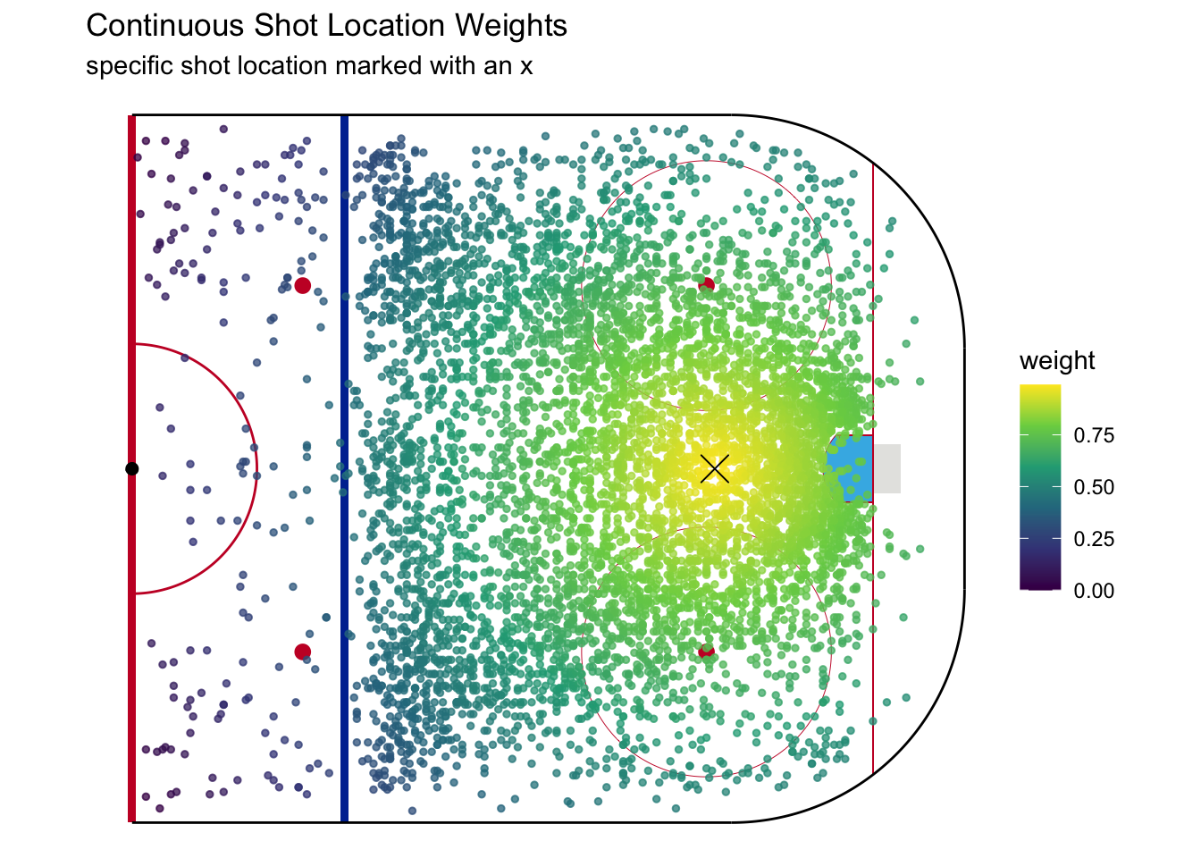
We’ve already come across a problem with this approach. Look at the weights above and think about geometry to see if you can spot it.

The problem is all the shots past the goal line and behind the blue line. Shots from behind the goal line are qualitatively different, due to the angle of the shot, from ones in front of the goal line. Similarly, shots from outside the zone are naturally much lower danger than those from just inside due to the way the game flows in the offensive versus neutral zone. We are building a continuous model, but in doing so we must account for how the geometry of the ice and rules of the game dictate discontinuities in expected goals. We will therefore pool shots from outside the offensive zone or a foot behind the goal line⁴ to be “outside the scoring zone” and share a single xG value, while the continuous xG model will be applied only between the blue line and goal line.

After that change, the calculation of expected goals is fairly straightforward. First, we assign a value of 1 of every goal and 0 for every non-goal shot in our sample. We multiply each shot’s result by its weight, and then we normalize the resulting product to a percentage that represents expected goals. Each shot’s expected goal value is the summed weights of all the goals in the sample divided by the total weight across all shots. The following figure shows the xG of every shot in our sample using this method.

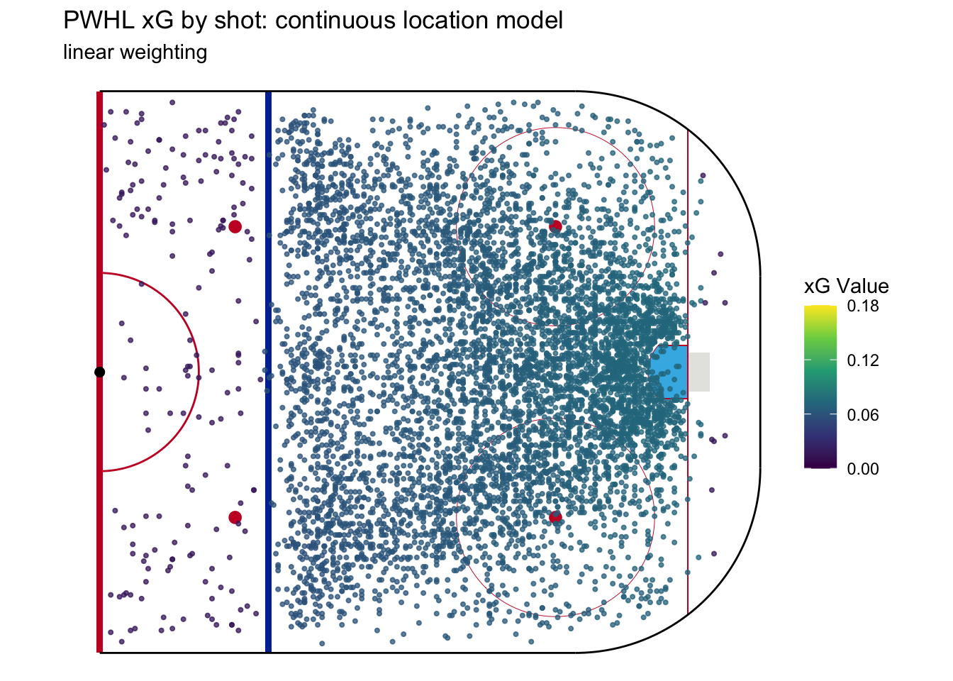
This is … underwhelming. The xG is pretty much identical for all shots. But the best thing about a weighted continuous model is that it introduces two tunable parameters that are not available to a discrete model. This means we have a lot more flexibility in building a good model.

The first parameter we can change is how the weighting is calculated. In the example above, the weights reduce linearly with distance. But we can change them to reduce by the distance squared. Consider 2 shots where the first is 5 feet away from the location we’re calculating xG for and the second is 10 feet away. If the weighting is linear, then the second shot gets half of much weight as the first. But by weighting on the squared distance, the second shot only gets a quarter the weight of the first.

Here’s what a squared weighting expected goal model looks like:

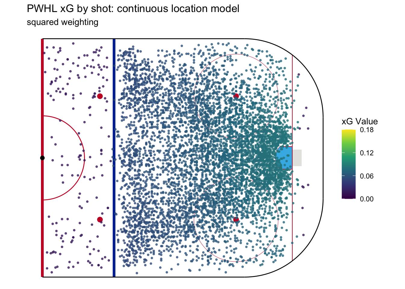
We can see now that the shots near the net have higher xG than the linear model and shots farther away have lower xG. In building and tuning a continuous model, we can choose any exponent by which the weighting is reduced. The higher the weighting exponent, the stronger this trend.

The second parameter brings back an element of the discrete models by setting a maximum distance within which shots are considered. The reason we’d do this is to ensure that shots don’t get credited xG they don’t deserve. For example, a shot from the point should probably not consider shots from next to the crease or, as a more extreme example, a shot from the defensive zone shouldn’t use anything from inside the zone as a basis to calculate xG. So we can specify a maximum distance (from the shot in question) within which past shots are used for calculating xG. More precisely, anything outside the maximum distance is given a weight of 0. The following model has a maximum distance cutoff of 44 feet, approximately the distance between the 2 faceoff dots in the offensive zone.

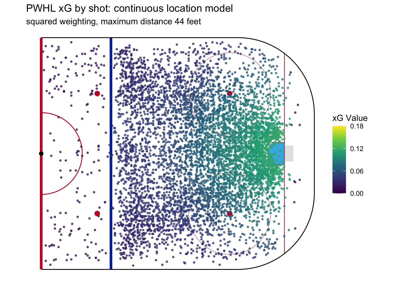
Now we see even stronger trends in xG. This is because the xG calculation for shots near the crease draws more exclusively from other shots near the crease instead of shots from the corner or near the point. Likewise, the xG calculation for point shots is more exclusively based on data that includes other point shots.

Now it’s time to turn our attention to balancing the two parameters. In general, max distance represents the tradeoff between sample size and accuracy. Set the max distance too small, and there won’t be enough shots in the sample to be confident in the xG estimates. Set the max distance too large, and some shots will be included in the xG calculation that shouldn’t be. The weighting exponent adjusts how sensitive the model is. A model that isn’t sensitive enough will assign nearly the same xG to every shot, as is the case with the linear model we saw above. But one that’s too sensitive can assign very different xG values to shots from nearly the same location.

Making the right model is about balance, especially because we have a fairly small sample. If we had a sample large enough to support both building and validating a model with precision, we could mathematically find the right balance. But I don’t think that’s feasible here.⁵ In playing around with various parameter settings, I learned a few things. Think of them as my three postulates about this type of location-based xG model:

1. The weighting exponent generally needs to be at least 3 to get the kind of sensitivity required to find specific dangerous areas of the ice. The plots we’ve seen so far, for example, essentially capture shot distance and only shot distance.

2. Models built using a larger distance parameter tend to overestimate expected goals. That is, the number of goals expected by the xG model far exceeds the number of actual goals scored. I think this is because larger distances include the prime scoring area for every shot, inflating expected goals from less dangerous areas of the ice.

3. The two parameters are not independent and can, in some ways, be used to achieve the same thing. For example, there’s no need to have a really small max distance and a very high weighting exponent.

With all of this in mind, I decided to start with a large distance and increase the exponent until the expected goals matched the observed goals pretty closely, and then vice versa. I found that making either value extreme didn’t work well, and landed on a middle ground of 25 feet for the maximum distance and the 5th power for the weighting exponent.

Here’s the resulting model, which is based based solely on shot location:

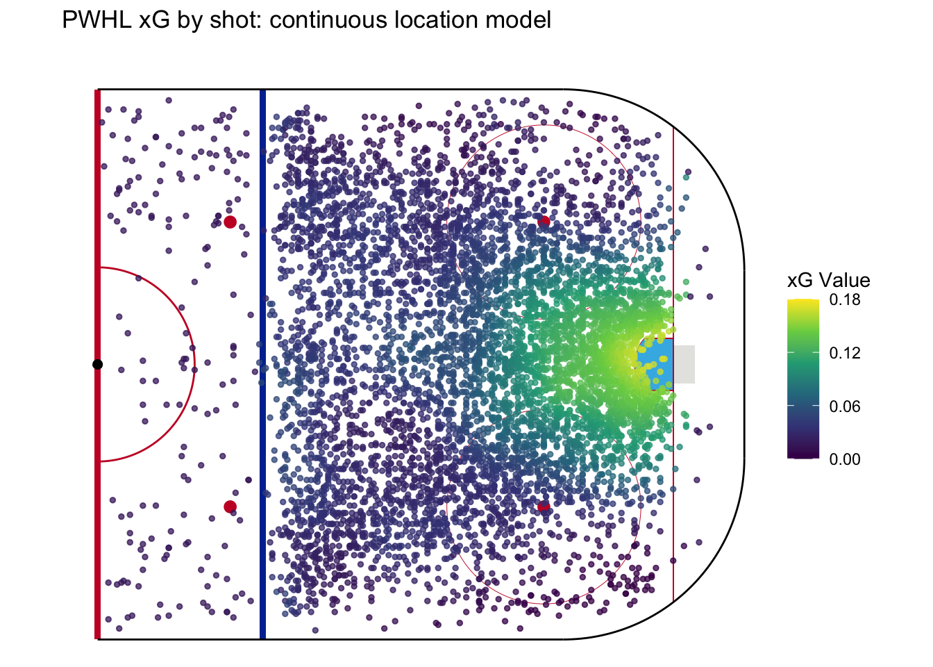
A good xG model is now starting to take shape. For example, once shots get beyond the faceoff dots, the model rewards those taken closer to the center of the ice. I think this makes sense - a point shot from the center of the ice has a better angle at the net, normally has more traffic in front of the goalie, and is closer to the net than shots taken from closer to the boards.

But this is not a finished model! We still have two predictors to incorporate in the next post: shot type and shot location. Let’s finish this post with something tangible: how this model, incomplete though it may be, ranks the six PWHL teams from last season.

NOTE: empty net shots and goals are excluded

	Actual Goals			Expected Goals
Team	For	Against	Share	For	Against	Share
MIN	82	73	52.9%	92.0	74.4	55.3%
OTT	60	70	46.2%	63.1	56.4	52.8%
TOR	79	66	54.5%	71.7	69.8	50.7%
MTL	69	66	51.1%	72.9	75.8	49.0%
BOS	67	76	46.9%	71.4	83.0	46.3%
NY	62	68	47.7%	58.5	70.3	45.4%

Footnotes

1. If you’re unsure what this means, review my first post.

2. Another issue to consider is that the PWHL shot location is accurate to within a foot, but isn’t perfect. Therefore, it’s tough to know if any shot within a foot or so of the home plate region’s boundaries was inside or outside. It shouldn’t matter much either way, but in the discrete location model it makes a big difference.

3. Remember that in calculating expected goals, we remove all shots taken on an empty net.

4. Why a foot behind the goal line? First, we know the shot location data is only accurate to within a foot or so. Second, shots from the goal line itself are more likely to be deflected in by the goalie or a defender or were intended as passes into the crease.

5. In fact, I think implementing some kind of more mathematical process for optimizing the parameters would likely result in overfitting.