My PWHL Expected Goals Model

making what I think is best

This is a series of posts in which I create an open-source PWHL model. We’ll calculate expected goals in various ways, create forecasts, and explore other things we could do with the model, like player ratings. If this sounds fun, you can follow along on Github here. When it’s ready and the PWHL season has begun, I’ll have a way to view and interact with the model on my website.

---

In my last PWHL post, we created an expected goals model that handles location data continuously instead of discretely. The next step is to incorporate more variables into this model framework. We’ve already identified the best candidates to be included in my first post from this series: shot type and shooter position (forward versus defender).

This post comes in three parts. First, we’ll discuss how to include these two discrete variables into a continuous xG model. Second, we’ll discuss covariance and whether or they should be included in the final model (this will be the most difficult part of the post). Third, we’ll do some analysis to finalize our PWHL expected goals model for the 2024-25 season.

Part 1: How to incorporate discrete variables into a continuous model

In my previous post, I made a key statement about why a continuous location-based xG model is important:

Hockey is not a discrete, categorical game and (I know this is mostly an aesthetic argument) I think xG models should reflect that.

This is not true of either shot type or shooter position. Both are discrete. A shot is either a tip or it’s not, and a shooter either plays forward or they don’t. I think it’s more intuitive to include them in discrete models, as in the first post, versus continuous models. To include them in a continuous model, there are two options.

1. We can use the same categorization approach for discrete variables as we did before. Accordingly, we group all shots into categories based on their shot type and shooter position and then apply the location-based calculation of xG only to shots in the sample that match the characteristics of the shot in question.

2. Instead of removing shots from the sample that don’t match the categorization, we increase the weight given to shots that do. All shots in the sample count, but those with more similar characteristics count more.¹

Suppose we’re calculating xG for a slap shot from a defender. In Option 1, we use the normal location-based xG calculation, but only do so only using other slap shots from defenders. In Option 2, we include all shots but increase the influence that other slap shots from defenders have on the xG calculation.

Option 2 is strictly better than Option 1.² In practice, Option 1 breaks our already small sample into even smaller discrete pieces. We are likely to run into the same bounding and resolution issues we encountered in my first post. Option 2 keeps the sample as large as possible and allows for flexibility in how the weighting increases. Getting back to our example, Option 2 allows us to increase the weight of all slap shots, not just those from defenders.

Implementing Option 2 is fairly straightforward. In my previous post from this series, we established that the continuous location xG model had two tunable parameters. The first was the weighting exponent which dictates how the weighting for shots in the sample is reduced with distance. The second was the maximum distance within which shots from the sample are given any weight. Now we add a third parameter - how much the weight of a sample shot is increased if it matches one of the characteristics of the shot considered.

To see how this changes things, we’ll start by plotting expected goals as we did in the last post, without accounting for either shot type or shooter position.

Now we can stack shot type and shooter position as predictors on top of this. In the following example, sample shots are weighted 10 times more if they match either the shot type or shooter position of the shot type in question. Sample shots that match both are given 100 times more weight.

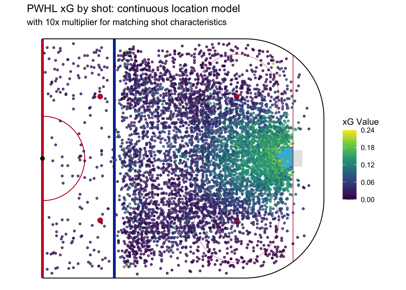
The location-only model showed a homogeneous view of xG in regard to shot location. The farther away, in any direction, the lower the xG. In the new model, there is now more heterogeneity in expected goals versus shot location. For example, there are some higher xG (roughly 0.1) shots near the blue line mixed in with the lower danger shots. These are slap shots from defenders, which we know can sometimes be high danger. Of all the models we’ve made so far in this series, I think this one best captures our intuitive sense what types of shots are high versus low danger.

This is great, but before rolling out the red carpet for this brave new xG model, we need to ask: is there such a thing as a model that’s too fancy? Or, in other words, we’ve spent enough time asking whether we could include these predictors that we now need to ask whether we should. Why or why not?

Part 2: Covariance and restraint

The reason to include more predictors³ in a model feels obvious - to make the model better! But including more predictors can quietly make a model worse, most often because of covariance. Covariance occurs when two variables or predictors have joint variability or move together.⁴ In terms of our xG model, we can understand covariance as occurring when two potential predictors share some common characteristic that influences expected goals.

Let’s consider the possible covariance between shot location and shot type. We’ve already seen in this series that slap shots tend to be the shot type with the lowest xG. Why? One explanation is that this is driven by some characteristics of slap shots themselves; for instance, they normally aren’t taken as quickly as snap or wrist shots so goalies have more time to get set. But it could simply be that slap shots tend to be taken farther away from the net. We know the truth is probably a mix of these two explanations, but the point is what this says about covariance. The first explanation would result in low covariance between shot type and shot location while the second would result in high covariance.

There are several ways to test for whether two variables are covaried. We won’t be talking about them in this post because they tend to be focused around hypothesis testing and generally don’t perform well when comparing discrete and continuous variables. Even more importantly, the existence of covariance doesn’t necessarily mean we shouldn’t use a variable as a model predictor. A little covariance is fine - in fact, it’s nearly impossible to avoid.

Instead, let’s set out an operational definition of what high and, more helpfully, low covariance looks like in practice. As we discussed, two variables are covaried when they move together. So, if we were to build a model using one of the two as a predictor, and then make a second model where both are predictors, we wouldn’t expect much change. Thinking in an extreme case might be helpful here - if we build a model based on shot location and then add shot location as a predictor again, we’ll get a (nearly) identical model.

When two highly covaried predictors are included in the same model, the model then doubles down on the characteristic(s) they share and often overfits the sample. An overfit model is one that fits its sample data too well - so well that it’s actually reflecting random variance within the sample. By modeling this specific randomness, overfit models perform poorly when used on new data. Getting back to our example - if slap shots are low danger only because they tend to be taken farther away from the net, including shot type as a predictor won’t make a location-based xG model much better. Going further, adding shot type as a predictor may also capture some random variability by accident and overfit the model.

Overfitting can be hard to spot. Adding a new predictor to a model can never make it perform worse on its sample data. Model fitting algorithms will always be able to give a useless predictor a coefficient of 0, effectively removing it from the model entirely. A true 0 is rare though, so adding another predictor to a model will always make it appear better in practice, even in the case of overfitting.

This brings us to the million-dollar question about modeling. Despite our original intuition, the million-dollar question is not: when we add either shot type or shooter position to an xG model, does it improve? The answer, of course, will always be yes. The true million-dollar question is more nuanced: when we add either shot type or shooter position to an xG model, does it improve enough to justify the increased risk of overfitting?

And so we land on a core idea of modeling: restraint. It’s tempting to create a fancy and sophisticated model that fits our sample data incredibly well. Our general cultural understanding of models is that complicated models are, by nature, better than simpler ones. This is incorrect. The best modelers balance the desire to include more predictors with the restraint to exclude predictors that don’t make our models better enough.

It’s time to shift from theory to practice by making some models, looking at the output, and determining whether we should add variables to the models or practice restraint.⁵

Part 3: Towards our final PWHL model

Our model evaluation will be results-based. We will compare the number of goals various xG models expect to be scored in our sample versus the number of goals actually scored. This will allow us to check if our expected goals models have, well, the right expectations. If adding a predictor creates a model that gets better at expecting the correct number of goals scored, there’s a very good chance that predictor is both valuable and isn’t too covaried with other predictors.

But we need to consider the role of randomness in this. Hockey is a random game and we know shooting percentages can fluctuate from season to season. In our sample, there were 419 goals. If a model expects 425 goals, we can all agree that’s a reasonable expectation. If a model expects only 300 goals, we can likewise agree that’s too far off. We quantitatively define what “a reasonable expectation” means by using confidence intervals. Confidence intervals provide a range within which the true number of expected goals should be based on our sample. If two models are well within the confidence interval, that means we don’t have the data needed to be able to clearly differentiate them. By extension, if one of these two models is closer to the observed number goals than the other, it can be a sign of overfitting.

Moving forward, we’ll be using the 90% confidence interval for the number of goals that should be expected given the number of goals scored in the sample. When we see a 90% confidence interval, that means there’s a 90% chance the true expected goals value falls within it. Put another way, there’s a 10% chance that it doesn’t. If you’re a bit confused, that’s fine. It will make a lot more sense once we get to a practical example.

Let’s start by looking at a model that uses only shot location versus one based on shot location plus shooter position. To make the impact of the new predictor clear, we’ll use a 100x weighting multiplier instead of the 10x we demonstrated earlier. The following plot shows the number of goals expected by each model. The horizontal lines and boxes indicate the observed number of goals in our sample and the surrounding 90% confidence interval. Because we want to evaluate if the model with shooter position as a predictor is better, we look at the results by shooter position.

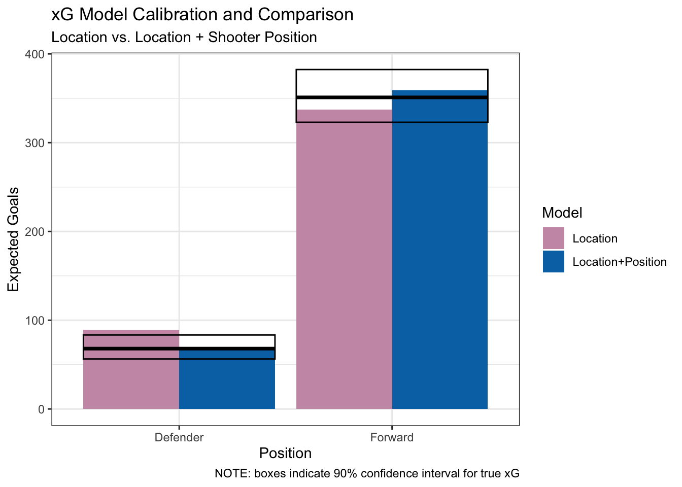
In this plot, we can see that the “Location+Position” model has more accurate expectations. Going from the “Location” model to “Location+Position” model brings the expectation for goals from defenders from outside the confidence interval to inside. The model improves for forwards too, but both models are well within the 90% confidence interval, so this improvement is just superficial. In some cases, getting closer to the true sample value while staying within the confidence interval is a warning sign for overfitting. Our conclusion regarding whether shooter position should be included as a predictor is inconclusive - it seems a bit better, but there’s some warning signs as well.

We’ll circle back to this in a bit, but for now let’s look at shot type:

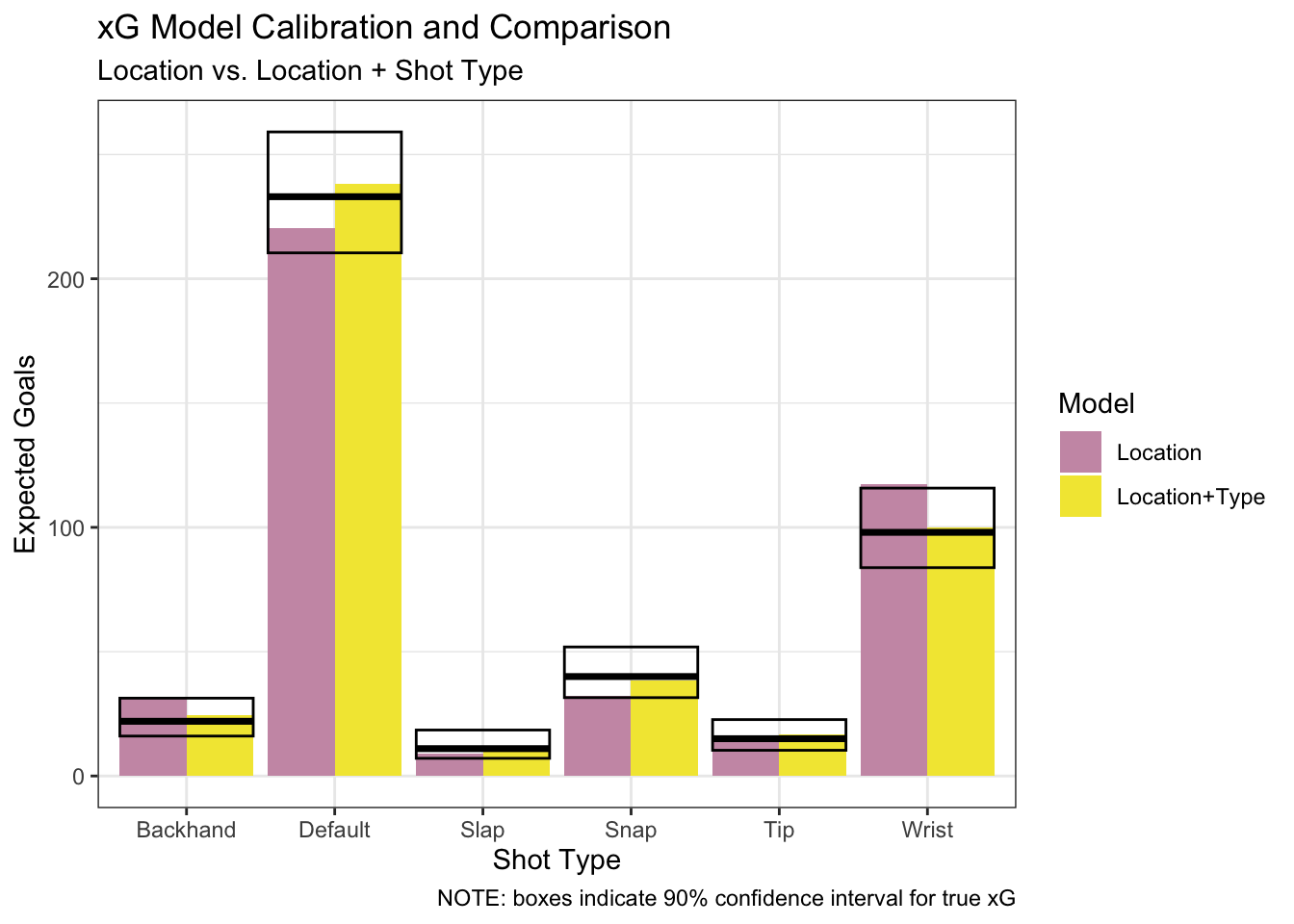
This is a very clear example of a model getting better by including a new predictor. Adding shot type brings model predictions from outside (or on the fringes of) the 90% confidence interval to inside of it for several shot types. The fact that the “Location” model is outside of so many confidence intervals on its own strongly suggests it’s not expecting the right things. On top of that, the consistent improvement across several shot types in the “Location+Type” model is a clear sign that shot type helps bring the expectations more in line. We know that our final xG model should account for shot type.

Because shot type is such a strong predictor, it is theoretically possible that the value in using shooter position was masked earlier by not including shot type. Now that we know for sure we are including shot type, we should revisit whether adding shooter position in this new context changes our original conclusion.

The next plot looks more complicated than the previous ones because it has both predictors, but we’re looking at all the same information. The question is whether the (green) “All Three” model outperforms the (yellow) “Location+Type” model.

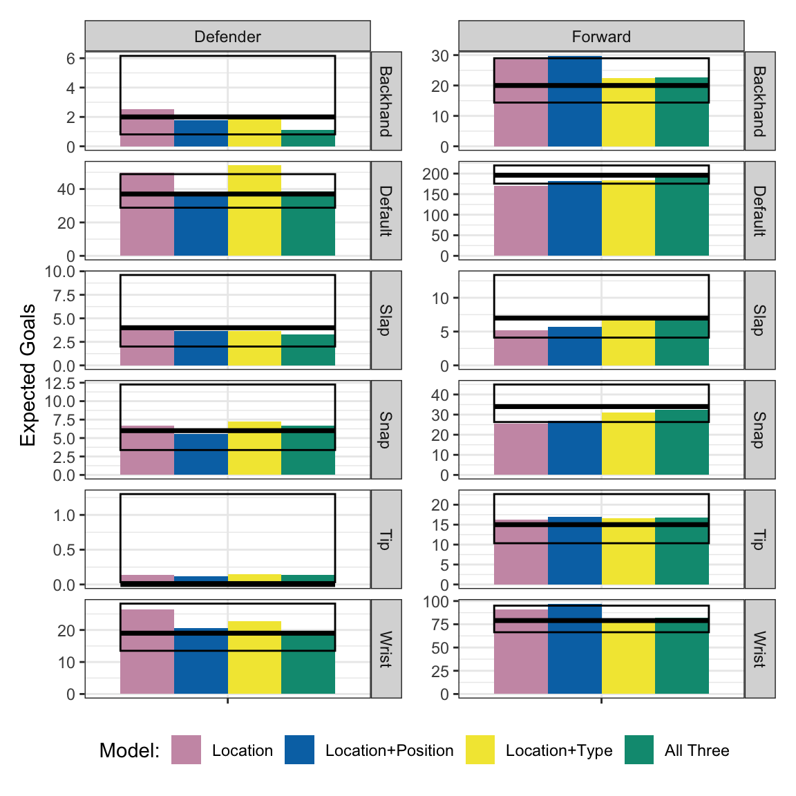
As we saw before, the model with shooter position doesn’t really change any predictions for forwards. But it does for defenders. The “default” shot type goes from well outside the confidence interval to dead on the number of observed goals. Wrist shots look better too. The “All Three” model undoubtedly matches the sample better than the “Location+Type” model.

But recall what we discussed in the previous section - this is true by definition. We return to finding balance - the million-dollar question isn’t whether the “All Three” model is better, it’s whether it’s better enough to risk overfitting.

I think the answer is no.⁶ The only significant improvement appears to be for default shots from defenders. That’s 1 out of 12 conditions in the model and a couple others (backhands from defenders) may get worse. Recall our definition of a 90% confidence interval - there’s a 10% chance the true expectation falls outside the sample confidence interval by random chance alone. Given there’s 12 conditions, we should expect a good xG model to miss the confidence interval on one or two of them. The “All Three” model doesn’t miss any.⁷ Given our small sample, this strongly suggests overfitting to me.

After rejecting shooter position for the second time (until we get more data), we have our final predictors: shot location and shot type.

The Final Model

With the final predictors chosen, we need to turn our focus to model tuning. Our model has three parameters, the first two of which we optimized in the last post. We have the weighting exponent which decreases the weight given to sample shots with distance, the maximum distance at which sample shots are used to calculate xG for any given shot, and the weight increase given to sample shots which match the shot type for any given shot.

In our first demonstration of this approach, we used a weight factor of 10; that is, we increased the weight given to matching shots tenfold. For the purposes of figuring out whether shot type was important, we used a weight factor of 100. What’s optimal?

I created a model for each weight factor from 10 to 200, incrementing by 10. To see what might be better, I plotted the average error in how many goals of each shot type were expected by the model versus what was observed. Here’s the results:

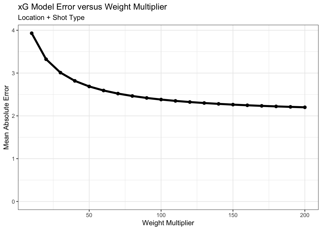
As the weight multiplier increases, the relative importance of shot type over shot location for calculating xG increases. Because we are evaluating the model accuracy by shot type, the model error decreases monotonically. Instead of choosing a near infinite weight, though, we should choose a weight that balances accuracy versus overfitting or removing the importance of shot location entirely. The average error starts to level off at around 2.5 goals, so I’m going to choose a weight multiplier halfway between 50 and 100: 75.

Here’s a look at our final PWHL expected goals model for the 2024-2025 season. This plot has every shot from the 2024 season colored by xG:

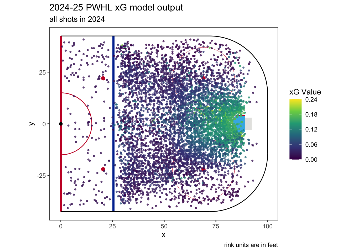
If you’re curious, the single shot with the highest xG value occurred in PWHL Game 40. It was between Ottawa and Toronto and taken almost exactly halfway through. On a transition play, Rosalie Demers took a snap shot right by the crease which had an xG value 0.237, or nearly a (modeled) 1 in 4 chance of being scored. It was saved.

That’s all for this one. Next up: using this expected goal model to calculate team ratings as we build towards making a predictive model.

Footnotes

1. //TODO: insert Animal Farm reference here

2. Mathematically speaking, the two are not so different as they appear. We treat discrete and continuous models as entirely different, but a discrete model is, in fact, a special case of a continuous model where all weights are forced to be either 0 or 1.

3. A quick note on some terminology. When we talk about characteristics available in our sample data, like shot type, we call them variables. Once we talk about variables being included in an xG model, we then call them predictors.

4. This definition comes straight from Wikipedia. If you have a decent mathematical background, Math Wikipedia is surprisingly an excellent place to learn more. Math Wikipedia articles tend to be well-written and focus on conceptual knowledge, often supported by great visualizations and a good example or two.

5. Once again, we could use mathematical tests to be precise in our evaluation, but in our case I don’t think this is the right thing to do. Hypothesis testing is a very different application of statistics than modeling and we should be careful crossing those tracks. Because of our smaller sample, they may not yield valid results. We will be better served using sound judgement from here, not blindly relying on tests which can be easily fooled.

6. That said, I think there are entirely rational arguments to prefer the “All Three” model (see the next footnote, for example). Without getting more data and out-of-sample testing, it’s a judgement call. The nice thing about modeling is that we can wait for more data to come in and revisit this conversation again with more clarity in the future.

7. We can be a bit more precise here. If our 90% confidence intervals are well-calibrated, and they should be given we’re using the Wilson Confidence Interval, then the odds of having all 12 conditions within the intervals is roughly 30%. Not super likely, but far from being significantly unlikely.